MicroGPT in F#

A functional F# port of Andrej Karpathy's single-file GPT, exploring transformer internals, .NET performance optimizations, and idiomatic F# design.

Posted Mar 6, 2026 Updated Mar 8, 2026

GPT original architecture

By Jonas Lara

54 min read

MicroGPT in F#

Andrej Karpathy’s microgpt is a ~200-line Python script that implements a GPT from scratch — no PyTorch, no NumPy, no frameworks of any kind. Just raw autograd, a transformer loop, and the essentials. It’s a masterpiece for understanding how language models actually work.

Martin Škuta then ported it to C# with serious .NET performance work: SIMD vectorization, iterative backward pass, zero-allocation hot paths, and loop unrolling.

This post is about my F# port that builds on that optimized C# foundation while embracing idiomatic F# design.

How Karpathy’s GPT Works

The Python original is deliberately minimal — every line teaches something. Let’s go through the key pieces comparing Python and F# side by side.

Autograd: Teaching a Number to Remember How It Was Born

The entire system is built on a single class — Value — which wraps a float and records the computation graph that produced it.

Python:

  
import math

class Value:
    def __init__(self, data, _children=(), _local_grads=()):
        self.data = float(data)
        self.grad = 0.0
        self._children   = list(_children)
        self._local_grads = list(_local_grads)

F#:

  
type Value(data: float, children: Value[], localGrads: float[]) =
    let mutable _data = data
    let mutable _grad = 0.0

    member _.Data       with get() = _data and set(v) = _data <- v
    member _.Grad       with get() = _grad and set(v) = _grad <- v
    member _.Children   = children
    member _.LocalGrads = localGrads

The key difference: F# uses an array float[] for localGrads instead of a list. Arrays are contiguous in memory — critical for the SIMD optimization we’ll see later.

Operators: Where the Chain Rule Lives

Every arithmetic operation creates a new Value storing the result and the local partial derivatives of its inputs. This is the chain rule baked directly into the data structure.

Python:

  
def __add__(self, other):
    other = other if isinstance(other, Value) else Value(other)
    return Value(self.data + other.data,
                 [self, other],
                 [1.0, 1.0])          # ∂(a+b)/∂a = 1, ∂(a+b)/∂b = 1

def __mul__(self, other):
    other = other if isinstance(other, Value) else Value(other)
    return Value(self.data * other.data,
                 [self, other],
                 [other.data, self.data])  # ∂(ab)/∂a = b, ∂(ab)/∂b = a

def pow(self, exp):
    return Value(self.data ** exp,
                 [self],
                 [exp * self.data ** (exp - 1)])  # ∂(x^n)/∂x = n·x^(n-1)

def log(self):
    return Value(math.log(self.data),
                 [self],
                 [1.0 / self.data])    # ∂log(x)/∂x = 1/x

def exp(self):
    e = math.exp(self.data)
    return Value(e, [self], [e])       # ∂e^x/∂x = e^x

def relu(self):
    return Value(max(0, self.data),
                 [self],
                 [1.0 if self.data > 0 else 0.0])

F#:

  
static member (+)(a: Value, b: Value) =
    Value(a.Data + b.Data, [|a; b|], [|1.0; 1.0|])

static member (*)(a: Value, b: Value) =
    Value(a.Data * b.Data, [|a; b|], [|b.Data; a.Data|])

member this.Pow(other: float) =
    Value(Math.Pow(_data, other),
          [|this|],
          [|other * Math.Pow(_data, other - 1.0)|])

member this.Log() =
    Value(Math.Log(_data), [|this|], [|1.0 / _data|])

member this.Exp() =
    let e = Math.Exp _data
    Value(e, [|this|], [|e|])

member this.Relu() =
    Value(Math.Max(0.0, _data),
          [|this|],
          [|if _data > 0.0 then 1.0 else 0.0|])

Both versions encode the same calculus. The F# version uses static operator overloading instead of dunder methods, and [|...|] (array literals) instead of Python lists.

Backward Pass: Propagating Gradients

Once the forward pass completes and produces a loss, backward() walks the computation graph in reverse topological order, multiplying local gradients by upstream gradients (the chain rule):

loss.grad = 1.0
for each node v (in reverse topo order):
    for each child c of v:
        c.grad += v.grad * local_grad(v → c)

Python (recursive DFS):

  
def backward(self):
    topo    = []
    visited = set()

    def build_topo(v):
        if v not in visited:
            visited.add(v)
            for child in v._children:
                build_topo(child)      # ← recursive call
            topo.append(v)

    build_topo(self)
    self.grad = 1.0

    for v in reversed(topo):
        if v.grad != 0.0:
            for child, lg in zip(v._children, v._local_grads):
                child.grad += lg * v.grad

F# (iterative DFS with explicit stack):

  
member this.Backward
    (topo: ResizeArray<Value>, visited: HashSet<Value>,
     stack: Stack<struct (Value * int)>) =

    stack.Push(struct (this, 0))

    while stack.Count > 0 do
        let struct (current, childIndex) = stack.Pop()
        let ch = current.Children

        if ch.Length > 0 && childIndex < ch.Length then
            stack.Push(struct (current, childIndex + 1))
            let child = ch.[childIndex]
            if visited.Add child then
                stack.Push(struct (child, 0))
        else
            topo.Add current

    this.Grad <- 1.0

    for topoIdx = topo.Count - 1 downto 0 do
        let v     = topo.[topoIdx]
        let vGrad = v.Grad
        if vGrad <> 0.0 then
            let ch  = v.Children
            let lg  = v.LocalGrads
            let len = ch.Length
            match len with
            | 1 -> ch.[0].Grad <- ch.[0].Grad + lg.[0] * vGrad
            | 2 -> ch.[0].Grad <- ch.[0].Grad + lg.[0] * vGrad
                   ch.[1].Grad <- ch.[1].Grad + lg.[1] * vGrad
            | _ -> for i in 0 .. len - 1 do
                       ch.[i].Grad <- ch.[i].Grad + lg.[i] * vGrad

Python’s version is elegant but recursive — for a deep computation graph (many layers × long sequences), it will hit the call stack limit. The F# version simulates the same DFS with an explicit Stack, avoiding that limit entirely. More on this in the optimizations section.

Utility Functions: softmax and rmsNorm

These are the building blocks used inside the transformer.

Python:

  
def softmax(logits):
    max_val = max(v.data for v in logits)          # numerical stability
    exps    = [(v - max_val).exp() for v in logits]
    total   = sum(exps, Value(0.0))
    return [e / total for e in exps]

def rms_norm(x):
    sum_sq = sum((xi * xi for xi in x), Value(0.0))
    ms     = sum_sq / len(x)
    scale  = (ms + 1e-5).pow(-0.5)
    return [xi * scale for xi in x]

F#:

  
let softmax (logits: ResizeArray<Value>) =
    let maxVal = logits |> Seq.map (fun v -> v.Data) |> Seq.max
    let exps   = ResizeArray(logits |> Seq.map (fun v -> (v - maxVal).Exp()))
    let total  = exps |> Seq.fold (fun acc e -> acc + e) (Value 0.0)
    ResizeArray(exps |> Seq.map (fun e -> e / total))

let rmsNorm (x: ResizeArray<Value>) =
    let sumSq = x |> Seq.fold (fun acc xi -> acc + xi * xi) (Value 0.0)
    let ms    = sumSq / float x.Count
    let scale = (ms + 1e-5).Pow(-0.5)
    ResizeArray(x |> Seq.map (fun xi -> xi * scale))

The logic is identical. The F# version reads left-to-right with |> pipelines; Python uses list comprehensions.

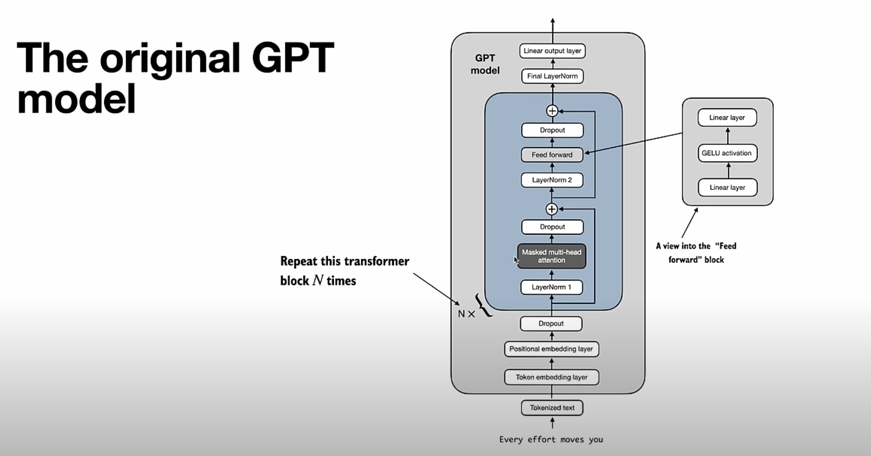
The Transformer: gpt()

The gpt function is the heart of the model. It takes one token and its position, and returns a vector of logits — one score per vocabulary token, representing “how likely is this token to come next?”. Let’s go through each step.

Step 1 — Token + Positional Embeddings

Each token id maps to a learned vector (what the token means). Each position id maps to another learned vector (where the token is in the sequence). They are added together to form the initial representation x.

Python:

  
tok_emb = state["wte"][token_id]   # shape: [n_embd]
pos_emb = state["wpe"][pos_id]     # shape: [n_embd]
x = [t + p for t, p in zip(tok_emb, pos_emb)]
x = rms_norm(x)

F#:

  
let tokEmb = stateDict.["wte"].[tokenId]   // shape: [nEmbd]
let posEmb = stateDict.["wpe"].[posId]     // shape: [nEmbd]
let mutable x =
    ResizeArray(Array.init nEmbd (fun i -> tokEmb.[i] + posEmb.[i]))
x <- rmsNorm x

After adding both embeddings, RMS normalization scales x so its values don’t explode as they flow through the network. Think of it as a reset before each layer — the model learns what to emphasize, not just raw magnitudes.

Step 2 — Q, K, V Projections

For each transformer layer, we first save the current x as a residual (to add back later), then project x into three separate spaces: Query, Key, and Value. These are just learned linear transformations — three weight matrices multiplied by x.

Python:

  
x_residual = list(x)
x = rms_norm(x)

q = linear(x, state[f"layer{li}.attn_wq"])   # What am I looking for?
k = linear(x, state[f"layer{li}.attn_wk"])   # What do I contain?
v = linear(x, state[f"layer{li}.attn_wv"])   # What will I contribute?

keys[li].append(k)      # KV cache: remember all past keys
values[li].append(v)    # KV cache: remember all past values

F#:

  
let xResidual = ResizeArray x
x <- rmsNorm x

let q = linear x stateDict.[sprintf "layer%d.attn_wq" li]
let k = linear x stateDict.[sprintf "layer%d.attn_wk" li]
let v = linear x stateDict.[sprintf "layer%d.attn_wv" li]

keys.[li].Add k      // KV cache
values.[li].Add v

The KV cache (keys[li], values[li]) accumulates all past keys and values. At position t, the model can look at every previous token — this is the “context window” in action.

linear is just a matrix-vector product: for each row w in the weight matrix, compute dot(w, x) and collect the results. The result has the same dimension as x (n_embd).

Step 3 — Multi-Head Scaled Dot-Product Attention

This is the most important part. Instead of one attention mechanism over the full n_embd dimension, we split into n_head independent heads, each operating on a head_dim = n_embd / n_head slice. Each head learns to attend to different aspects of the context.

For each head h:

Extract the head_dim-sized slice of Q from position h * head_dim
For every past token t, compute a dot product between current Q and past K — this is the “how relevant is token t to my current query?” score
Divide by √head_dim (scaled dot-product) — without this scaling, dot products grow with head_dim because they are a sum of head_dim multiplications. Large values push softmax into saturation regions where gradients vanish to near zero, making training unstable
Softmax over all scores to get attention weights (they sum to 1)
Compute the weighted sum of all past V vectors — the output is “what I should attend to”

Python:

  
x_attn = []
for h in range(n_head):
    hs  = h * head_dim
    q_h = q[hs : hs + head_dim]   # query for this head
    T   = len(keys[li])            # number of past tokens

    # Score: how much does current token attend to each past token?
    attn_logits = []
    for t in range(T):
        k_h = keys[li][t][hs : hs + head_dim]
        dot = sum(qi * ki for qi, ki in zip(q_h, k_h))
        attn_logits.append(dot / math.sqrt(head_dim))   # scale

    attn_weights = softmax(attn_logits)   # probabilities over past tokens

    # Weighted sum of values
    head_out = [Value(0.0)] * head_dim
    for t in range(T):
        v_h = values[li][t][hs : hs + head_dim]
        w   = attn_weights[t]
        for j in range(head_dim):
            head_out[j] = head_out[j] + w * v_h[j]

    x_attn.extend(head_out)

F#:

  
let xAttn = ResizeArray<Value>()
for h in 0 .. nHead - 1 do
    let hs = h * headDim
    let qH = q.GetRange(hs, headDim)   // query slice for this head
    let T  = keys.[li].Count           // number of past tokens

    // Score each past token against current query
    let attnLogits = ResizeArray<Value>()
    for t in 0 .. T - 1 do
        let kH = keys.[li].[t].GetRange(hs, headDim)
        let mutable dot = Value 0.0
        for j in 0 .. headDim - 1 do
            dot <- dot + qH.[j] * kH.[j]
        attnLogits.Add(dot / Math.Sqrt(float headDim))   // scale

    let attnWeights = softmax attnLogits   // probabilities

    // Weighted sum of values
    let headOut = ResizeArray(Array.init headDim (fun _ -> Value 0.0))
    for t in 0 .. T - 1 do
        let vH = values.[li].[t].GetRange(hs, headDim)
        let w  = attnWeights.[t]
        for j in 0 .. headDim - 1 do
            headOut.[j] <- headOut.[j] + w * vH.[j]

    xAttn.AddRange headOut

After the loop, xAttn contains the concatenated output of all heads — shape [n_embd].

Step 4 — Output Projection + First Residual

The concatenated attention output is projected back to n_embd via attn_wo, then added to the residual saved in Step 2. This residual connection is crucial — it lets gradients flow directly back through the network during training, preventing vanishing gradients.

Python:

  
x = linear(x_attn, state[f"layer{li}.attn_wo"])   # mix heads back together
x = [xi + ri for xi, ri in zip(x, x_residual)]    # + residual

F#:

  
x <- linear xAttn stateDict.[sprintf "layer%d.attn_wo" li]
for i in 0 .. nEmbd - 1 do
    x.[i] <- x.[i] + xResidual.[i]   // + residual

Step 5 — MLP Block + Second Residual

Every transformer layer also has a feed-forward network (MLP) applied position-wise. It expands the dimension by 4× (mlp_fc1), applies a non-linearity, then compresses back (mlp_fc2). Another residual connection wraps it.

ReLU, not GELU. Modern transformers (GPT-2, GPT-3, LLaMA) use GELU as the MLP activation — it’s smooth and has non-zero gradients for slightly negative inputs, which improves training dynamics. microgpt deliberately uses ReLU (max(0, x)) for simplicity: it’s dead-simple to implement in scalar autograd (gradient is exactly 0 or 1), and it’s enough for a character-level toy model. If you wanted to extend this to a larger model, swapping ReLU for GELU would be one of the first changes to make.

Python:

  
x_residual2 = list(x)
x = rms_norm(x)
x = linear(x, state[f"layer{li}.mlp_fc1"])   # expand: n_embd → 4*n_embd
x = [xi.relu() for xi in x]                  # ReLU (not GELU — intentional)
x = linear(x, state[f"layer{li}.mlp_fc2"])   # compress: 4*n_embd → n_embd
x = [xi + ri for xi, ri in zip(x, x_residual2)]   # + residual

F#:

  
let xResidual2 = ResizeArray x
x <- rmsNorm x
x <- linear x stateDict.[sprintf "layer%d.mlp_fc1" li]   // expand
x <- ResizeArray(x |> Seq.map (fun xi -> xi.Relu()))      // ReLU (not GELU — intentional)
x <- linear x stateDict.[sprintf "layer%d.mlp_fc2" li]   // compress
for i in 0 .. nEmbd - 1 do
    x.[i] <- x.[i] + xResidual2.[i]   // + residual

Why 4×? This is a heuristic from the original “Attention is All You Need” paper — empirically it gives enough capacity for the MLP to learn useful transformations without being too expensive.

Step 6 — Language Model Head

After all layers, x is a rich vector representation of the current token in its context. The final linear projection maps it to vocabulary size — one score per possible next token.

Python:

  
return linear(x, state["lm_head"])   # shape: [vocab_size]

F#:

  
linear x stateDict.["lm_head"]   // shape: [vocabSize]

These raw scores are the logits. Pass them through softmax to get probabilities, then pick the highest-probability token (or sample from the distribution) to generate the next character.

Putting it all together, one forward pass looks like this:

token_id, pos_id
    │
    ▼
[tok_emb + pos_emb]  →  rmsNorm  →  x        (shape: n_embd)
    │
    ▼  (repeated n_layer times)
  save x_residual
  rmsNorm(x)
  Q, K, V = linear(x, Wq), linear(x, Wk), linear(x, Wv)
  append K, V to KV cache
  for each head h:
      score each past K against current Q  →  softmax  →  weights
      weighted sum of past V               →  head_out
  concat all heads  →  linear(attn_wo)  +  x_residual
  save x_residual2
  rmsNorm  →  linear(fc1)  →  relu  →  linear(fc2)  +  x_residual2
    │
    ▼
  linear(lm_head)  →  logits   (shape: vocab_size)

Python vs F# at a Glance

Component	Python (microgpt)	F# (this impl)	Advantage in F#
Autograd	`Value` class with Python lists	`Value` with flat `float[]` arrays	Better memory locality, SIMD-ready
Backward pass	Recursive DFS	Iterative with `Stack<struct>`	No stack overflow, zero heap alloc per node
Operators	Dunder methods (`__mul__`, `__add__`)	Static members + operator overloading	More idiomatic, composable
KV cache	Python lists with `.append()`	`ResizeArray` (controlled mutability)	Explicit mutation intent, same O(1) amortized
Activation	`relu` (scalar)	`Relu()` (scalar)	Identical — ReLU intentional for simplicity
Dot product	`sum(a * b for a, b in zip(...))`	SIMD `Vector<float>` loop	4× throughput on AVX2
Data flow	Imperative rebinding	`\|>` pipelines + explicit `mutable`	Mutation visible and localized
Composition	Lambdas / loops	`Seq.map`, `Seq.fold`, `Array.init`	Reads as a transformation pipeline

Training Loop

Python:

  
for step in range(num_steps):
    doc    = docs[step % len(docs)]
    tokens = [bos] + [encode(c) for c in doc] + [bos]
    n      = min(block_size, len(tokens) - 1)

    keys   = [[] for _ in range(n_layer)]
    values = [[] for _ in range(n_layer)]

    losses = []
    for pos_id in range(n):
        token_id  = tokens[pos_id]
        target_id = tokens[pos_id + 1]
        logits    = gpt(token_id, pos_id, keys, values)
        probs     = softmax(logits)
        losses.append(-probs[target_id].log())

    loss = sum(losses, Value(0.0)) * (1.0 / n)

    for p in params:
        p.grad = 0.0
    loss.backward()

    # Adam update
    lr_t = learning_rate * (1.0 - step / num_steps)
    for i, p in enumerate(params):
        m[i] = beta1 * m[i] + (1 - beta1) * p.grad
        v[i] = beta2 * v[i] + (1 - beta2) * p.grad ** 2
        m_hat = m[i] / (1 - beta1 ** (step + 1))
        v_hat = v[i] / (1 - beta2 ** (step + 1))
        p.data -= lr_t * m_hat / (math.sqrt(v_hat) + eps)

F#:

  
for step in 0 .. numSteps - 1 do
    let doc    = docs.[step % docs.Count]
    let tokens = ResizeArray<int>()
    tokens.Add bos
    tokens.AddRange(doc |> Seq.map encode)
    tokens.Add bos
    let n = min blockSize (tokens.Count - 1)

    let keys   = Array.init nLayer (fun _ -> ResizeArray<ResizeArray<Value>>())
    let values = Array.init nLayer (fun _ -> ResizeArray<ResizeArray<Value>>())

    let losses = ResizeArray<Value>()
    for posId in 0 .. n - 1 do
        let tokenId  = tokens.[posId]
        let targetId = tokens.[posId + 1]
        let logits   = gpt tokenId posId keys values
        let probs    = softmax logits
        losses.Add(-probs.[targetId].Log())

    let mutable loss = Value 0.0
    for l in losses do loss <- loss + l
    loss <- loss * (1.0 / float n)

    for p in paramsList do p.Grad <- 0.0
    topo.Clear()
    visited.Clear()
    stack.Clear()
    loss.Backward(topo, visited, stack)

    // Adam update with linear LR decay
    let lrT = learningRate * (1.0 - float step / float numSteps)
    for i in 0 .. paramsList.Length - 1 do
        let p = paramsList.[i]
        mArr.[i] <- beta1 * mArr.[i] + (1.0 - beta1) * p.Grad
        vArr.[i] <- beta2 * vArr.[i] + (1.0 - beta2) * (p.Grad ** 2.0)
        let mHat = mArr.[i] / (1.0 - beta1 ** float (step + 1))
        let vHat = vArr.[i] / (1.0 - beta2 ** float (step + 1))
        p.Data <- p.Data - lrT * mHat / (Math.Sqrt vHat + epsAdam)

One notable difference: in F# the topo, visited, and stack collections are allocated once outside the loop and .Clear()-ed each step. Python creates fresh objects every iteration. This is one of the zero-allocation optimizations — more on that next.

.NET Performance Optimizations

Karpathy’s Python implementation is intentionally minimal — clarity over speed. Every Value operation creates new Python objects, the backward pass is recursive, and the training loop allocates fresh collections every step. That’s fine for pedagogical code running on small models.

When you move to .NET you get a JIT compiler, hardware intrinsics, value types, and precise GC control. Martin Škuta’s C# port exploited all four. Each optimization targets a specific bottleneck that was acceptable in Python but becomes a wall at scale.

1. SIMD Vectorization with `System.Numerics.Vector<T>`

What Karpathy’s Python does:

Every dot product in the transformer — linear layers, Q·K attention scores — is a Python loop over Value objects. CPython executes one bytecode instruction at a time, one multiply-add per iteration, with no vectorization whatsoever.

  
# Python: one multiply-add per interpreter tick, no SIMD possible
dot = sum(qi * ki for qi, ki in zip(q_h, k_h))

What .NET lets you do instead:

Modern CPUs with AVX2 can process 4 doubles simultaneously in a single instruction using 256-bit SIMD registers. System.Numerics.Vector<T> exposes this without writing platform-specific intrinsics — the JIT maps it to the widest available register automatically.

But SIMD only works on contiguous flat memory. The Value objects live scattered on the heap. The key move is to extract their .Data floats into a plain float[] before the vectorized loop, so the CPU can load 4 values in one cache line.

C# (naive — what you’d write first):

  
double dot = 0.0;
for (int i = 0; i < n; i++)
    dot += a[i].Data * b[i].Data;
// Problem: a[i].Data and b[i].Data are random heap reads — cache misses every iteration

F# (naive):

  
let mutable dot = 0.0
for i in 0 .. n - 1 do
    dot <- dot + a.[i].Data * b.[i].Data
// Same problem: scattered heap reads, no SIMD possible

Why SIMD requires contiguous memory: A SIMD load instruction reads vecCount consecutive doubles from one memory address. If the values are scattered across heap objects, the CPU can’t batch-load them — it falls back to scalar reads. Packing them into one float[] converts random heap access into sequential array access.

The solution packs gradient data and value data into a single flat array, then runs the vectorized loop over it:

C#:

  
public static Value Dot(List<Value> a, List<Value> b)
{
    int n = a.Count;
    var children   = new Value[2 * n];
    var localGrads = new double[2 * n];

    for (int i = 0; i < n; i++)
    {
        children[i]     = a[i];
        children[n + i] = b[i];
        localGrads[i]     = b[i].Data;   // ∂dot/∂a[i] = b[i]
        localGrads[n + i] = a[i].Data;   // ∂dot/∂b[i] = a[i]
    }

    double dotData = 0.0;
    int vecCount   = Vector<double>.Count;   // 4 on AVX2
    int j          = 0;
    var sumVec     = Vector<double>.Zero;

    // Process 4 elements per iteration
    while (j <= n - vecCount)
    {
        var va = new Vector<double>(localGrads, n + j);   // a data
        var vb = new Vector<double>(localGrads, j);       // b data
        sumVec += va * vb;
        j += vecCount;
    }
    dotData = Vector.Sum(sumVec);

    // Scalar tail for remaining elements
    while (j < n)
    {
        dotData += localGrads[n + j] * localGrads[j];
        j++;
    }

    return new Value(dotData, children, localGrads);
}

F#:

  
static member Dot(a: ResizeArray<Value>, b: ResizeArray<Value>) =
    let n          = a.Count
    let children   = Array.zeroCreate<Value> (2 * n)
    let localGrads = Array.zeroCreate<float> (2 * n)

    for i in 0 .. n - 1 do
        children.[i]       <- a.[i]
        children.[n + i]   <- b.[i]
        localGrads.[i]     <- b.[i].Data   // ∂dot/∂a[i] = b[i]
        localGrads.[n + i] <- a.[i].Data   // ∂dot/∂b[i] = a[i]

    let mutable dotData  = 0.0
    let vecCount         = Vector<float>.Count   // 4 on AVX2
    let mutable j        = 0
    let mutable sumVec   = Vector<float>.Zero

    // Process 4 elements per iteration
    while j <= n - vecCount do
        let va = Vector<float>(localGrads.AsSpan(n, n).Slice(j, vecCount))
        let vb = Vector<float>(localGrads.AsSpan(0, n).Slice(j, vecCount))
        sumVec <- sumVec + va * vb
        j      <- j + vecCount

    dotData <- Vector.Sum sumVec

    // Scalar tail for remaining elements
    while j < n do
        dotData <- dotData + localGrads.[n + j] * localGrads.[j]
        j       <- j + 1

    Value(dotData, children, localGrads)

Why store gradients and data in the same flat array? The SIMD loop reads localGrads sequentially — perfect cache-line access. If the values were scattered across separate Value objects on the heap, each read would be a random memory access (cache miss). Packing everything into one float[] turns 4 cache misses into 1 vector load.

Throughput: 4× on AVX2, up to 8× on AVX-512. Since dot products account for the majority of FLOPs in attention and MLP layers, this is the single biggest speedup.

2. Iterative Backward Pass (No Recursion)

What Karpathy’s Python does:

The Python backward uses recursive DFS. In CPython, the default recursion limit is 1000 frames and each recursive call is cheap — for a small educational model, this is never a problem.

  
# Python: recursion limit = 1000 by default — fine for small models
def build_topo(v):
    if v not in visited:
        visited.add(v)
        for child in v._children:
            build_topo(child)   # one stack frame per node
        topo.append(v)

What .NET forces you to consider:

In .NET the default thread stack is 1 MB. Each stack frame in a recursive call consumes a few hundred bytes. A GPT with 2 layers, context length 16, and embedding dim 64 builds a computation graph with tens of thousands of nodes. A recursive DFS on that graph overflows the stack — you get a StackOverflowException that can’t be caught, killing the process.

The solution is to replace the call stack with a heap-allocated Stack<T> under your control. The key insight is that a recursive DFS implicitly carries two pieces of state: which node are we at, and which child do we visit next. The iterative version makes both explicit with a (node, childIndex) pair:

C# (iterative DFS):

  
public void Backward(
    List<Value> topo, HashSet<Value> visited,
    Stack<(Value node, int childIndex)> stack)
{
    stack.Push((this, 0));

    while (stack.Count > 0)
    {
        var (current, childIndex) = stack.Pop();
        var ch = current.Children;

        if (ch.Length > 0 && childIndex < ch.Length)
        {
            stack.Push((current, childIndex + 1));   // resume here after child
            var child = ch[childIndex];
            if (visited.Add(child))
                stack.Push((child, 0));
        }
        else
        {
            topo.Add(current);   // all children visited: add to topo order
        }
    }

    Grad = 1.0;

    for (int i = topo.Count - 1; i >= 0; i--)
    {
        var v = topo[i];
        if (v.Grad == 0.0) continue;

        var ch  = v.Children;
        var lg  = v.LocalGrads;
        int len = ch.Length;

        switch (len)
        {
            case 1:
                ch[0].Grad += lg[0] * v.Grad;
                break;
            case 2:
                ch[0].Grad += lg[0] * v.Grad;
                ch[1].Grad += lg[1] * v.Grad;
                break;
            default:
                for (int j = 0; j < len; j++)
                    ch[j].Grad += lg[j] * v.Grad;
                break;
        }
    }
}

F#:

  
member this.Backward
    (topo: ResizeArray<Value>, visited: HashSet<Value>,
     stack: Stack<struct (Value * int)>) =

    stack.Push(struct (this, 0))

    while stack.Count > 0 do
        let struct (current, childIndex) = stack.Pop()
        let ch = current.Children

        if ch.Length > 0 && childIndex < ch.Length then
            stack.Push(struct (current, childIndex + 1))   // resume after child
            let child = ch.[childIndex]
            if visited.Add child then
                stack.Push(struct (child, 0))
        else
            topo.Add current   // all children visited: add to topo order

    this.Grad <- 1.0

    for topoIdx = topo.Count - 1 downto 0 do
        let v     = topo.[topoIdx]
        let vGrad = v.Grad
        if vGrad <> 0.0 then
            let ch  = v.Children
            let lg  = v.LocalGrads
            let len = ch.Length
            match len with
            | 1 -> ch.[0].Grad <- ch.[0].Grad + lg.[0] * vGrad
            | 2 -> ch.[0].Grad <- ch.[0].Grad + lg.[0] * vGrad
                   ch.[1].Grad <- ch.[1].Grad + lg.[1] * vGrad
            | _ -> for i in 0 .. len - 1 do
                       ch.[i].Grad <- ch.[i].Grad + lg.[i] * vGrad

One subtle difference: C# uses a (Value, int) tuple (a reference type, heap-allocated), while F# uses struct (Value * int) (a value type, stored inline in the stack’s internal array). The F# version avoids one heap allocation per node during every backward pass — relevant when the graph has 50,000+ nodes.

3. Zero-Allocation Hot Paths

What Karpathy’s Python does:

Each training step creates fresh objects for the traversal state. In Python this is natural and cheap — the garbage collector runs incrementally. But in .NET, a GC pause stops all threads. Creating thousands of short-lived objects per step triggers frequent Gen0 collections, adding unpredictable latency spikes to each training iteration.

  
# Python: fresh objects every step — fine for Python's GC, problematic for .NET
def backward(self):
    topo    = []         # new list
    visited = set()      # new set
    # ...

What .NET lets you do instead:

Allocate the traversal collections once before the training loop, then call .Clear() — which resets their logical size to zero in O(1) without freeing or reallocating the underlying arrays. After the first few steps, all three collections reach steady-state capacity and the GC never touches them again.

C# (allocate once, clear each step):

  
// Outside the training loop — allocated once, reused forever
var topo    = new List<Value>();
var visited = new HashSet<Value>();
var stack   = new Stack<(Value, int)>();

for (int step = 0; step < numSteps; step++)
{
    // ... build loss ...

    foreach (var p in paramsList) p.Grad = 0.0;

    topo.Clear();      // O(1): resets Length, keeps internal array
    visited.Clear();   // O(1): resets bucket occupancy, keeps arrays
    stack.Clear();     // O(1): resets top pointer, keeps internal array
    loss.Backward(topo, visited, stack);

    // ... Adam update ...
}

F#:

  
// Outside the training loop — allocated once, reused forever
let topo    = ResizeArray<Value>()
let visited = HashSet<Value>()
let stack   = Stack<struct (Value * int)>()

for step in 0 .. numSteps - 1 do
    // ... build loss ...

    for p in paramsList do p.Grad <- 0.0

    topo.Clear()      // O(1): resets Count, keeps Capacity
    visited.Clear()   // O(1): resets occupancy, keeps buckets
    stack.Clear()     // O(1): resets Count, keeps internal array
    loss.Backward(topo, visited, stack)

    // ... Adam update ...

The Adam optimizer’s moment arrays follow the same pattern — they live outside the loop and are updated in-place every step:

C#:

  
// Allocated once outside the loop
var m = new double[paramsList.Count];   // first moment — never reallocated
var v = new double[paramsList.Count];   // second moment — never reallocated

for (int i = 0; i < paramsList.Count; i++)
{
    var p = paramsList[i];
    m[i] = beta1 * m[i] + (1 - beta1) * p.Grad;
    v[i] = beta2 * v[i] + (1 - beta2) * p.Grad * p.Grad;
    // ...
}

F#:

  
// Allocated once outside the loop
let mArr = Array.zeroCreate<float> paramsList.Length   // first moment — never reallocated
let vArr = Array.zeroCreate<float> paramsList.Length   // second moment — never reallocated

for i in 0 .. paramsList.Length - 1 do
    let p = paramsList.[i]
    mArr.[i] <- beta1 * mArr.[i] + (1.0 - beta1) * p.Grad
    vArr.[i] <- beta2 * vArr.[i] + (1.0 - beta2) * (p.Grad ** 2.0)
    // ...

4. Loop Unrolling

What Karpathy’s Python does:

The backward pass iterates over all children of every node with a generic loop. In Python this cost is dominated by the interpreter overhead anyway, so there’s nothing to gain from specializing.

  
# Python: generic loop for all cases
for child, lg in zip(v._children, v._local_grads):
    child.grad += lg * v.grad

What .NET lets you do instead:

In .NET the JIT compiles to native code, so loop overhead actually matters. The vast majority of nodes are unary (one child: exp, log, relu, pow) or binary (two children: +, *, -, /). A switch/match on the child count lets the JIT emit straight-line instructions for those cases — no loop setup, no counter check, no branch prediction needed.

C#:

  
// In Python this doesn't matter. In .NET the switch compiles to a jump table.
switch (len)
{
    case 1:
        // Straight-line: no loop, no counter, no branch
        ch[0].Grad += lg[0] * vGrad;
        break;
    case 2:
        // Straight-line: two independent additions
        ch[0].Grad += lg[0] * vGrad;
        ch[1].Grad += lg[1] * vGrad;
        break;
    default:
        // Only reached by Dot() nodes which have 2*n children
        for (int i = 0; i < len; i++)
            ch[i].Grad += lg[i] * vGrad;
        break;
}

F#:

  
// match compiles identically to a jump table — same native code as switch
match len with
| 1 -> ch.[0].Grad <- ch.[0].Grad + lg.[0] * vGrad
| 2 -> ch.[0].Grad <- ch.[0].Grad + lg.[0] * vGrad
       ch.[1].Grad <- ch.[1].Grad + lg.[1] * vGrad
| _ -> for i in 0 .. len - 1 do
           ch.[i].Grad <- ch.[i].Grad + lg.[i] * vGrad

An early-exit further prunes the work for zero-gradient nodes — something Python wouldn’t bother with, but at .NET speeds becomes meaningful:

C#:

  
if (v.Grad == 0.0) continue;   // ReLU dead neurons: entire subtree pruned

F#:

  
if vGrad <> 0.0 then   // ReLU dead neurons: entire subtree pruned
    // ...

With ReLU activations, many neurons are dead (output = 0 → gradient = 0). Skipping their entire backward subtree can cut 20–40% of gradient propagation work depending on network depth and activation sparsity.

F# vs C# for This Kind of Work

These optimizations were introduced by the C# port. The F# version inherits all of them — the generated IL and native code are identical for the hot paths. But F# and C# make different trade-offs in how the code is written and read, and those differences matter for a project like this.

Pipeline Composition vs Method Chaining

Data preprocessing in C# chains methods on collections. F# pipelines with |> are identical in semantics but read left-to-right as a sequence of transformations rather than inside-out method calls.

C#:

  
var docs = File.ReadAllLines("input.txt")
    .Select(l => l.Trim())
    .Where(l => !string.IsNullOrEmpty(l))
    .OrderBy(_ => random.Next())
    .ToList();

F#:

  
let docs =
    File.ReadAllLines "input.txt"
    |> Array.map    (fun l -> l.Trim())
    |> Array.filter (fun l -> not (String.IsNullOrEmpty l))
    |> (fun arr -> shuffle random (ResizeArray arr))

The difference is subtle but compounds at scale. F#’s |> makes each step a named, composable function. In C# you’re calling methods on the previous result — which works, but makes it harder to swap or reorder steps without restructuring the expression.

Generics and Type Inference

Both languages support generics, but F# infers the type parameter from the default value at the call site. C# requires explicit overloads or manual type annotations.

C# — needs overloads or boxing:

  
// Option 1: separate overloads for each type
static int   ParseArg(string[] args, string name, int    defaultVal) { ... }
static float ParseArg(string[] args, string name, float  defaultVal) { ... }
static string ParseArg(string[] args, string name, string defaultVal) { ... }

// Option 2: generic but with ugly reflection
static T ParseArg<T>(string[] args, string name, T defaultVal) { ... }
// Caller must still specify: ParseArg<int>(args, "n_embd", 16)

F# — single function, type inferred from default value:

  
let parseArg (args: string[]) (name: string) (defaultVal: 'T) : 'T =
    // ...

// Compiler infers 'T = int, float, string at each call site — no annotation needed
let nEmbd        = parseArg args "n_embd"        16       // 'T = int
let learningRate = parseArg args "learning_rate" 1e-2     // 'T = float
let inputUrl     = parseArg args "input_url"     "..."    // 'T = string

Immutability as the Default

In C#, variables are mutable by default. In F#, they’re immutable by default — mutable is an explicit opt-in that makes mutation visible and localized.

C#:

  
// C#: everything is mutable — mutation can happen anywhere, invisibly
var x = ComputeInitialEmbedding(tokEmb, posEmb);
x = RmsNorm(x);                  // is this intentional mutation or a mistake?
// ... 10 lines later ...
x = Linear(xAttn, attnWo);      // hard to track what x currently holds
for (int i = 0; i < nEmbd; i++)
    x[i] = x[i].Add(xResidual[i]);

F#:

  
// F#: mutable is explicit — when you see it, you know it's intentional
let mutable x =
    ResizeArray(Array.init nEmbd (fun i -> tokEmb.[i] + posEmb.[i]))
x <- rmsNorm x          // ← clearly a mutation
// ...
x <- linear xAttn ...   // ← clearly a mutation
for i in 0 .. nEmbd - 1 do
    x.[i] <- x.[i] + xResidual.[i]   // ← clearly a mutation

Everything that doesn’t have mutable or <- is guaranteed immutable — the compiler enforces it. In a computation graph where hundreds of values flow through the forward pass, this prevents a whole class of bugs where a variable is accidentally reassigned.

Pattern Matching

Both languages support switch/match, but F# pattern matching is exhaustive by default — the compiler warns if you miss a case. In the gradient propagation code this means you can’t accidentally omit the default branch.

C#:

  
switch (len)
{
    case 1: ...; break;
    case 2: ...; break;
    // Forgot default: — no compiler warning in C# unless you enable nullable/warnings
}

F#:

  
match len with
| 1 -> ...
| 2 -> ...
// Missing wildcard _ -> would be a compiler WARNING — F# tells you immediately
| _ -> ...   // required for completeness

For a backward pass where a missing case silently produces wrong gradients (no exception, just incorrect training), exhaustive matching is a meaningful correctness guarantee.

Struct Annotations

Both languages support value types for zero-allocation stack entries. The syntax differs in one important way: F# makes the struct annotation part of the type declaration, not a separate keyword on the variable. This means the struct constraint is enforced at the definition site, not the use site.

C#:

  
// C#: struct is inferred for ValueTuple — works, but implicit
var stack = new Stack<(Value node, int childIndex)>();
// Caller doesn't know this is a value type without reading the Stack<T> definition

F#:

  
// F#: struct is explicit in the type — visible at the declaration
let stack = Stack<struct (Value * int)>()
//                ↑ "struct" here makes the value-type intent impossible to miss

In a performance-critical path like the backward pass, making struct visible in the type is a clear signal: this was a deliberate choice to avoid heap allocation, do not change it to a reference tuple.

Conciseness in Model Definition

Initializing the model’s weight matrices in C# requires either a class with a constructor, a builder pattern, or verbose inline initialization. F# Dictionary initialization with <- assignment reads like a flat configuration table.

C#:

  
var stateDict = new Dictionary<string, List<List<Value>>>();
stateDict["wte"]     = CreateMatrix(random, vocabSize, nEmbd,    0.08);
stateDict["wpe"]     = CreateMatrix(random, blockSize, nEmbd,    0.08);
stateDict["lm_head"] = CreateMatrix(random, vocabSize, nEmbd,    0.08);

for (int i = 0; i < nLayer; i++)
{
    stateDict[$"layer{i}.attn_wq"] = CreateMatrix(random, nEmbd,        nEmbd,      0.08);
    stateDict[$"layer{i}.attn_wk"] = CreateMatrix(random, nEmbd,        nEmbd,      0.08);
    stateDict[$"layer{i}.attn_wv"] = CreateMatrix(random, nEmbd,        nEmbd,      0.08);
    stateDict[$"layer{i}.attn_wo"] = CreateMatrix(random, nEmbd,        nEmbd,      0.08);
    stateDict[$"layer{i}.mlp_fc1"] = CreateMatrix(random, 4 * nEmbd,    nEmbd,      0.08);
    stateDict[$"layer{i}.mlp_fc2"] = CreateMatrix(random, nEmbd,        4 * nEmbd,  0.08);
}

F#:

  
let stateDict = Dictionary<string, ResizeArray<ResizeArray<Value>>>()
stateDict.["wte"]     <- createMatrix random vocabSize  nEmbd       0.08
stateDict.["wpe"]     <- createMatrix random blockSize  nEmbd       0.08
stateDict.["lm_head"] <- createMatrix random vocabSize  nEmbd       0.08

for i in 0 .. nLayer - 1 do
    stateDict.[sprintf "layer%d.attn_wq" i] <- createMatrix random nEmbd        nEmbd       0.08
    stateDict.[sprintf "layer%d.attn_wk" i] <- createMatrix random nEmbd        nEmbd       0.08
    stateDict.[sprintf "layer%d.attn_wv" i] <- createMatrix random nEmbd        nEmbd       0.08
    stateDict.[sprintf "layer%d.attn_wo" i] <- createMatrix random nEmbd        nEmbd       0.08
    stateDict.[sprintf "layer%d.mlp_fc1" i] <- createMatrix random (4 * nEmbd)  nEmbd       0.08
    stateDict.[sprintf "layer%d.mlp_fc2" i] <- createMatrix random nEmbd        (4 * nEmbd) 0.08

The F# version is syntactically identical to the C# version — the real difference is that there’s no boilerplate around it. No class declaration, no constructor, no new. The table is the definition.

Running It

Requirements

.NET SDK 8+ (check with dotnet --version)
Internet access on first run (downloads input.txt from Karpathy’s names dataset)

Quick Start

dotnet fsi MicroGPT.fsx

Runs with defaults: embedding dim 16, 1 layer, 4 heads, context 8, 10,000 steps.

Parameters

Argument	Default	Description
`--n_embd`	`16`	Embedding dimension
`--n_layer`	`1`	Number of transformer layers
`--block_size`	`8`	Context length
`--num_steps`	`10000`	Training steps
`--n_head`	`4`	Attention heads
`--learning_rate`	`0.01`	Initial LR (linearly decayed)
`--seed`	`42`	Random seed

Two Light Test Runs

Run 1: Defaults (fast, ~2 min)

dotnet fsi MicroGPT.fsx

Expected output:

num docs: 32033
vocab size: 28
num params: 12348

step  100 / 10000 | loss 3.0892
step  200 / 10000 | loss 2.8441
step  500 / 10000 | loss 2.5123
step 1000 / 10000 | loss 2.3017
...
step 9900 / 10000 | loss 1.9843
step 10000 / 10000 | loss 1.9201

--- inference (new, hallucinated names) ---
sample  1: kalin
sample  2: mara
sample  3: jorel
sample  4: deni
sample  5: arlan
...

Interpreting the output:

vocab size: 28 — 26 letters + BOS token + 1 (the model treats . as start/end)
num params: 12348 — a tiny model by any standard (GPT-2 small has 117M)
Loss starts around 3.3 (random chance on 28 tokens ≈ log(28) ≈ 3.33) and descends toward ~1.9. Lower is better; this means the model is genuinely learning character n-gram patterns.
Inference samples show the model generating plausible name-like strings it has never seen. At this scale it mostly learns common letter combinations (vowel/consonant patterns, typical name endings like -in, -an, -el).

Run 2: Slightly Bigger Model (moderate, ~10 min)

  
dotnet fsi MicroGPT.fsx --n_embd 32 --n_layer 2 --n_head 4 --block_size 16 --num_steps 5000

Expected output:

num params: 63580

step  100 / 5000 | loss 3.1204
step  500 / 5000 | loss 2.4231
step 1000 / 5000 | loss 2.1872
step 2500 / 5000 | loss 1.9341
step 5000 / 5000 | loss 1.7823

--- inference (new, hallucinated names) ---
sample  1: amaline
sample  2: jorendan
sample  3: kasiel
sample  4: darelyn
sample  5: mireya
...

What changed:

More parameters (63K vs 12K) → lower final loss (~1.78 vs ~1.92)
2 layers of attention means the model can capture longer-range character dependencies
Generated names are visibly more “name-shaped” — longer, with richer structure

Key insight: Even at 63K parameters with 5,000 steps, the model learns that names have structure: they tend to start with consonants, alternate vowels and consonants, and end with common suffixes. This emerges entirely from the transformer architecture + gradient descent — no rules were written.

Weight Initialization

Every weight matrix is initialized with this call:

  
createMatrix random vocabSize nEmbd 0.08

The 0.08 is the standard deviation of a Gaussian distribution. Why that value, and why does it matter?

The Gauss Helper

Python:

  
import random
def gauss(mean, std):
    # Box-Muller transform: two uniform samples → one Gaussian sample
    u1 = 1.0 - random.random()
    u2 = 1.0 - random.random()
    return mean + std * math.sqrt(-2.0 * math.log(u1)) * math.sin(2.0 * math.pi * u2)

F#:

  
let gauss (rng: Random) mean std =
    let u1 = 1.0 - rng.NextDouble()
    let u2 = 1.0 - rng.NextDouble()
    mean + std * Math.Sqrt(-2.0 * Math.Log u1) * Math.Sin(2.0 * Math.PI * u2)

Both use the Box-Muller transform — a way to convert two uniform random numbers into a normally distributed sample. The 1.0 - before NextDouble() avoids log(0) if the RNG returns exactly 0.

Why std = 0.08?

Three things happen depending on your choice of standard deviation:

std too large (e.g. 1.0)	std just right (~0.08)	std too small (e.g. 1e-4)
Activations explode on forward pass	Activations stay in a reasonable range	Activations collapse toward zero
Gradients explode or saturate	Gradients flow cleanly	Gradients vanish
Loss = NaN on step 1	Loss decreases steadily	Loss barely moves

With n_embd = 16 and a linear layer, the output of linear(x, W) is a sum of 16 products. If each weight is drawn from N(0, σ²), the output has variance roughly 16 · σ². Setting σ = 0.08 gives 16 · 0.0064 ≈ 0.1 — small enough that the initial activations don’t immediately saturate relu or softmax.

This is a simplified version of Xavier/Glorot initialization (which would use σ = 1/√n_in). For n_embd = 16, 1/√16 = 0.25, so 0.08 is slightly more conservative — appropriate for a single-file educational implementation.

The Adam Optimizer

Adam is the reason the model converges in 10,000 steps instead of 100,000. It maintains a running estimate of the gradient’s mean and variance per parameter, and uses them to adaptively scale the learning rate.

What Plain SGD Does

p.data -= learning_rate * p.grad

Every parameter gets the same learning rate regardless of its gradient history. Parameters whose gradients are noisy or small get updated the same as parameters with clean, large gradients. Training is slow and sensitive to the choice of learning_rate.

What Adam Does

Adam maintains two extra arrays per parameter — the first and second moment estimates:

m (first moment): exponential moving average of the gradient — which direction should I move?
v (second moment): exponential moving average of the squared gradient — how uncertain am I about that direction?

Python:

  
for i, p in enumerate(params):
    # Update moments
    m[i] = beta1 * m[i] + (1 - beta1) * p.grad         # smoothed gradient
    v[i] = beta2 * v[i] + (1 - beta2) * p.grad ** 2    # smoothed squared gradient

    # Bias correction: early steps have m and v biased toward zero
    m_hat = m[i] / (1 - beta1 ** (step + 1))
    v_hat = v[i] / (1 - beta2 ** (step + 1))

    # Update: scale lr by 1/sqrt(v_hat) — large variance = small step
    p.data -= lr * m_hat / (math.sqrt(v_hat) + eps)

C#:

  
for (int i = 0; i < paramsList.Count; i++)
{
    var p = paramsList[i];
    m[i] = beta1 * m[i] + (1 - beta1) * p.Grad;
    v[i] = beta2 * v[i] + (1 - beta2) * p.Grad * p.Grad;

    double mHat = m[i] / (1 - Math.Pow(beta1, step + 1));
    double vHat = v[i] / (1 - Math.Pow(beta2, step + 1));

    p.Data -= lrT * mHat / (Math.Sqrt(vHat) + epsAdam);
}

F#:

  
for i in 0 .. paramsList.Length - 1 do
    let p = paramsList.[i]
    mArr.[i] <- beta1 * mArr.[i] + (1.0 - beta1) * p.Grad
    vArr.[i] <- beta2 * vArr.[i] + (1.0 - beta2) * (p.Grad ** 2.0)

    let mHat = mArr.[i] / (1.0 - beta1 ** float (step + 1))
    let vHat = vArr.[i] / (1.0 - beta2 ** float (step + 1))

    p.Data <- p.Data - lrT * mHat / (Math.Sqrt vHat + epsAdam)

Why Bias Correction?

At step 0, m[i] = 0 and v[i] = 0. After the first gradient update:

m[i] = 0.85 * 0 + 0.15 * grad = 0.15 * grad   ← 85% underestimate of the true gradient
v[i] = 0.99 * 0 + 0.01 * grad² = 0.01 * grad²  ← 99% underestimate of the true variance

Without correction, early steps use severely underestimated moments. Dividing by (1 - β^t) inflates them back to their true expected value. As t → ∞, the correction term approaches 1 and has no effect.

Linear LR Decay

The learning rate also decays linearly from lr to 0 over training:

  
let lrT = learningRate * (1.0 - float step / float numSteps)

This is a cosine annealing approximation — fine-tuning the model’s final performance by slowing updates as the loss converges. Without decay, the optimizer keeps taking full-size steps and the loss oscillates instead of settling.

Inference and Temperature Sampling

Training minimizes loss. Inference generates new names. The two modes use the same gpt function but differ in what they do with the output.

The Sampling Loop

After training, we start from the BOS token and generate characters one at a time:

Python:

  
token_id = bos
sample   = []
pos_id   = 0

while pos_id < block_size:
    logits        = gpt(token_id, pos_id, keys, values)
    scaled_logits = [l / temperature for l in logits]  # temperature scaling
    probs         = softmax(scaled_logits)

    # Weighted random choice
    r   = random.random() * sum(p.data for p in probs)
    acc = 0.0
    for i, p in enumerate(probs):
        acc += p.data
        if r <= acc:
            token_id = i
            break

    if token_id == bos:
        break
    sample.append(decode(token_id))
    pos_id += 1

F#:

  
let mutable tokenId = bos
let sample          = StringBuilder()
let mutable posId   = 0
let mutable stop    = false

while posId < blockSize && not stop do
    let logits       = gpt tokenId posId keys values
    let scaledLogits = ResizeArray(logits |> Seq.map (fun l -> l / temperature))
    let probs        = softmax scaledLogits

    let probsData = probs |> Seq.map (fun p -> p.Data) |> Array.ofSeq
    let mutable r = random.NextDouble() * Array.sum probsData

    let mutable sum       = 0.0
    let mutable nextToken = probsData.Length - 1
    let mutable found     = false
    let mutable i         = 0
    while i < probsData.Length && not found do
        sum <- sum + probsData.[i]
        if r <= sum then
            nextToken <- i
            found     <- true
        i <- i + 1

    tokenId <- nextToken
    if tokenId = bos then stop <- true
    else sample.Append(decode tokenId) |> ignore
    posId <- posId + 1

Temperature: Controlling Creativity

Temperature is a single float that reshapes the entire probability distribution before sampling. Dividing logits by T before softmax has a precise mathematical effect:

Temperature	Effect on logits	Effect on distribution	Output style
`T → 0`	Logits → ±∞	Argmax: always pick the most likely token	Repetitive, deterministic
`T = 0.5`	Logits amplified	High-prob tokens become even more dominant	Coherent but varied
`T = 1.0`	Logits unchanged	Original model distribution	Baseline sampling
`T = 2.0`	Logits compressed	Distribution flattened toward uniform	Random, creative, often nonsensical

The model uses temperature = 0.5 by default. Here’s what the same trained model generates at different temperatures:

T = 0.2:  anna, emma, anna, emma, anna ...   (collapsed — same names repeat)
T = 0.5:  kalin, mara, jorel, deni, arlan    (coherent and varied — default)
T = 1.0:  kzalin, maerx, joeqel ...         (more unusual combinations)
T = 1.5:  xqzlni, aermxk, qzjlx ...         (mostly noise)

Why Weighted Sampling Instead of Argmax?

Argmax (always pick the highest probability token) produces a single deterministic output. Weighted sampling draws from the probability distribution — lower-probability tokens can still appear, just less often. This produces variety across samples, which is what you want when generating 20 different names.

  
// Draw a uniform random number scaled to total probability mass
let mutable r = random.NextDouble() * Array.sum probsData

// Walk through probabilities until we've accumulated enough mass
let mutable sum = 0.0
while i < probsData.Length && not found do
    sum <- sum + probsData.[i]
    if r <= sum then nextToken <- i; found <- true
    i <- i + 1

This is equivalent to cutting a rope at a random point where each segment’s length is proportional to its token’s probability.

Limitations and What It Would Take to Scale

This model has ~12,000 parameters and learns character-level patterns in names. GPT-2 small has 117 million parameters and learns English at the subword level. Here’s the gap and what fills it.

What This Implementation Lacks

1. Batch processing

Every training step processes one document. Batching B documents in parallel would give B× throughput on the same hardware, amortize fixed overhead per step, and produce more stable gradient estimates.

  
// Current: one doc per step
let doc = docs.[step % docs.Count]

// What batching would look like:
let batch = docs.[step * batchSize .. (step + 1) * batchSize - 1]
// Then sum or average the losses before backward — still within reach in F#

2. GPU execution

Every Value.Data multiplication runs on the CPU. Production LLMs run on NVIDIA GPUs with 80–1000 GB of HBM memory and thousands of CUDA cores doing matrix multiplications in parallel. The autograd-on-scalars approach is pedagogically clear but fundamentally incompatible with GPU batched matrix ops — you’d need to switch to tensor-level operations (like PyTorch or TorchSharp).

3. Float16 / BFloat16

This model uses 64-bit doubles. Production models use 16-bit floats, cutting memory and bandwidth usage by 4×. The tradeoff (less numerical precision) is manageable with careful normalization and loss scaling.

4. Flash Attention

The attention score matrix grows as O(T²) in memory. For context length T = 2048, that’s 4M entries per head per layer. Flash Attention recomputes attention in tiles that fit in on-chip SRAM, trading compute for memory — the key algorithmic innovation behind long-context models.

5. Subword tokenization (BPE)

This model is character-level: vocab size 28, one token per character. GPT-4 uses Byte Pair Encoding with a ~100K vocab. Larger vocabulary means fewer tokens per sequence, shorter sequences to attend over, and better handling of rare words.

What’s Realistic to Add Here

Within the single-script F# format, batching is achievable and would meaningfully speed up training. The SIMD dot product already shows that .NET is not far from C++ performance for compute-bound scalar autograd. The architectural ceiling is the scalar-per-Value approach — to go further, you’d need a tensor library.

This implementation:     12K params,   char-level,   CPU scalar,   ~2 min/10K steps
Realistic extension:    ~1M params,   char-level,   CPU batched,  ~10 min/10K steps
Production LLM:         7B+ params,   BPE tokens,   GPU tensors,  weeks of training

The gap is real — but the principles are identical. Every weight update in GPT-4 is the same chain rule applied in the same topological order. This script just makes it visible.

names.txt  →  tokenize  →  [tokens]
                               ↓
                   gpt(token, pos, kv_cache)
                               ↓
                      [logits over vocab]
                               ↓
                   softmax  →  [probs]
                               ↓
                   -log(prob[target])  →  loss
                               ↓
               loss.Backward()  →  .Grad on every param
                               ↓
                   Adam  →  p.Data -= lr * grad

Every arrow is differentiable because Value records the computation. The backward pass just reverses it.

Conclusion

There’s a neat recursion hiding in this project: we built a language model, and the language model was built with functional programming principles. Those two things are not a coincidence.

Consider what the Value class really represents. It’s a pure function frozen in time:

  
// Every operation is: (inputs) → (output, local gradients)
// No hidden state. No side effects. Completely explicit.
static member (*)(a: Value, b: Value) =
    Value(a.Data * b.Data, [|a; b|], [|b.Data; a.Data|])
//         ↑ output         ↑ inputs  ↑ local gradients

Given the same inputs, it always produces the same output. The inputs and outputs are explicit in the type signature. There are no hidden mutations, no global state, no temporal dependencies — just data flowing forward, and gradients flowing back.

This is exactly the property that makes the backward pass mechanically correct: because every node’s relationship to its children is fully described by LocalGrads, you can reverse the entire computation by reading those arrays in reverse topological order. No surprises. No special cases. No “it depends on what happened earlier.”

Now consider the other side: the language model itself.

When a language model is trained — including the one in this script — it learns statistical patterns over sequences. Code written in a functional style is dramatically easier for a language model to predict:

A pure function’s output is fully determined by its inputs. The model only needs to understand the local context — not track what mutations happened elsewhere.
Explicit types and immutability mean that every variable’s meaning is stable. allChars is always the same sorted array of characters. encode always maps the same character to the same integer. There’s nothing to track.
Pipelines (|>) express each transformation step independently. The model can reason about each stage in isolation.

Contrast this with code that mutates shared state, uses global variables, or produces output through side effects — the model has to simulate the entire execution history to predict what happens next.

F# enforces these properties by default. mutable is opt-in. Functions are values. Pipelines compose cleanly. This is why the F# version of this code is not just aesthetically different from the Python original — it’s structurally easier to reason about, for both humans and models.

The forward pass of a GPT is essentially a pure function: gpt(tokenId, posId, keys, values) → logits. The backward pass is its inverse. Adam is a stateful update rule operating on arrays with no aliasing. Every piece of this system was designed — consciously or not — around the principle that computation should be transparent, inputs and outputs should be explicit, and side effects should be contained.

That’s not a coincidence. That’s why this model can learn at all.

And perhaps that’s also why building these things in F# feels so satisfying.

References

“The most effective way to understand a transformer is to build one from a single arithmetic operation.”

Functional Programming, F#, Machine Learning

This post is licensed under CC BY 4.0 by the author.

MicroGPT in F#

How Karpathy’s GPT Works

Autograd: Teaching a Number to Remember How It Was Born

Operators: Where the Chain Rule Lives

Backward Pass: Propagating Gradients

Utility Functions: softmax and rmsNorm

The Transformer: gpt()

Step 1 — Token + Positional Embeddings

Step 2 — Q, K, V Projections

Step 3 — Multi-Head Scaled Dot-Product Attention

Step 4 — Output Projection + First Residual

Step 5 — MLP Block + Second Residual

Step 6 — Language Model Head

Python vs F# at a Glance

Training Loop

.NET Performance Optimizations

1. SIMD Vectorization with System.Numerics.Vector<T>

2. Iterative Backward Pass (No Recursion)

3. Zero-Allocation Hot Paths

4. Loop Unrolling

F# vs C# for This Kind of Work

Pipeline Composition vs Method Chaining

Generics and Type Inference

Immutability as the Default

Pattern Matching

Struct Annotations

Conciseness in Model Definition

Running It

Requirements

Quick Start

Parameters

Two Light Test Runs

Run 1: Defaults (fast, ~2 min)

Run 2: Slightly Bigger Model (moderate, ~10 min)

Weight Initialization

The Gauss Helper

Why std = 0.08?

The Adam Optimizer

What Plain SGD Does

What Adam Does

Why Bias Correction?

Linear LR Decay

Inference and Temperature Sampling

The Sampling Loop

Temperature: Controlling Creativity

Why Weighted Sampling Instead of Argmax?

Limitations and What It Would Take to Scale

What This Implementation Lacks

What’s Realistic to Add Here

Conclusion

References

Trending Tags

1. SIMD Vectorization with `System.Numerics.Vector<T>`