Algorithms and complexity
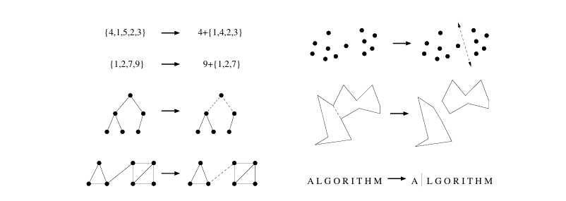
The algorithm is a step-by-step procedure, which defines a set of instructions that will be executed in a certain order to obtain the desired output. Algorithms are usually created independently of the underlying languages, that is, an algorithm can be implemented in more than one programming language.
Characteristics of an algorithm
Not all procedures can be called algorithms. An algorithm must have the following characteristics:
- Unambiguous: It must be clear and unambiguous. Each of its steps (or phases), and its inputs/outputs must be clear and must lead to a single meaning
- Input: Must have 0 or more well-defined inputs
- Output: Must have 1 or more well-defined outputs and must match the desired output
- Finiteness: Must finish after a finitive number of steps
- Feasibility: Must be feasible to execute with the available resources
- Standalone: Should have step-by-step instructions, which should be independent of any programming code
Algorithm design
In algorithm design and analysis, the second method is generally used to describe an algorithm. It makes it easy for the analyst to analyze the algorithm by ignoring all the unwanted definitions. You can observe what operations are being used and how the process flows, we design an algorithm to obtain a solution to a given problem. A problem can be solved in more than one way; therefore, many solution algorithms can be derived for a given problem, then the next step is to analyze the proposed solution algorithms and implement the best suitable solution.
Algorithm analysis
The efficiency of an algorithm can be analyzed in two different stages, before implementation and after implementation. They are the following:
- A priori analysis: This is a theoretical analysis of an algorithm. The efficiency of an algorithm is measured by assuming that all other factors, for example, processor speed, are constant and have no effect on the implementation
- A posteriori analysis: This is an empirical analysis of an algorithm. The selected algorithm is implemented using the programming language. This runs on the target computer’s machine. In this analysis, actual statistics such as runtime and space required are collected
Algorithmic complexity
Complexity theory is the study of the number of resources that an algorithm requires when running based on the size of its input, it is essential to know it to write code efficiently, there are two types of complexity:
Space complexity: It is the amount of memory an algorithm uses to run
Time complexity: It is the amount of time an algorithm takes to run, it is usually expressed in Big O notation
Asymptotic notation
Asymptotic notation is the language that allows us to analyze the execution time of an algorithm by identifying its behavior as the input size for the algorithm increases, there are different types of notations, but to improve in the study of algorithms for the moment you should only focus on the Big-O notation because it is an upper limit in the function, this limit represents worst-case behavior.
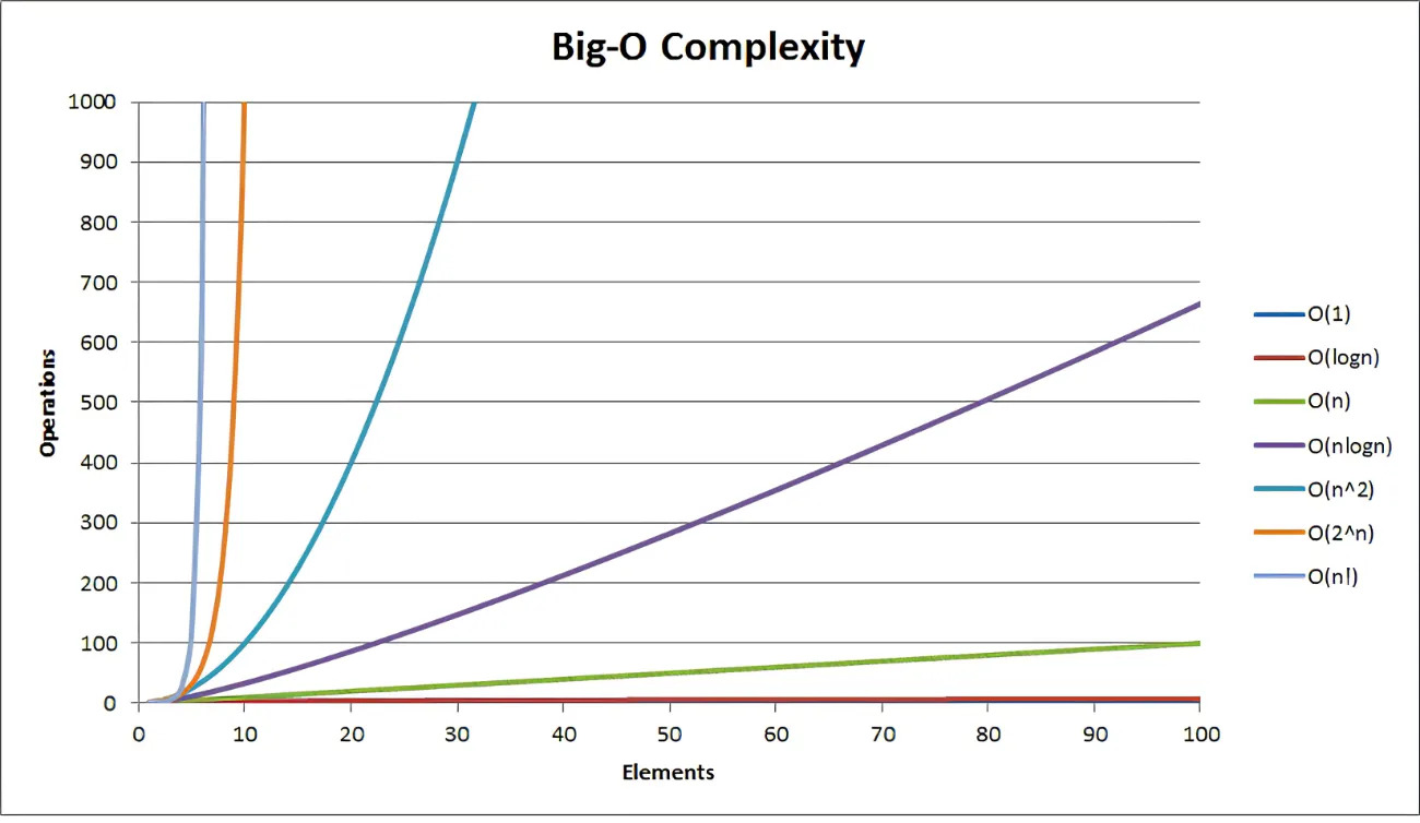 Big-O notation
Constant time complexity - O(1)
- Constant Time Complexity O(1) → An algorithm is said to run in constant time if it requires the same amount of time, regardless of input size, for example, accessing any element of an array or a function to exchange two numbers.
Algorithm for swap two values implemented in C:
1
2
3
4
5
6
7
8
void swap(int *a, int *b)
{
    int tmp;

     tmp = *a;
    *a = *b;
    *b = tmp;
}
Logarithmic time complexity O(log n)
- Logarithmic time complexity O(log n) → essentially means that the operating time grows in logarithmic proportion to that of the input size, i.e. the ratio of the number of operations N to the size of the input n decreases when the input size increases, e.g. the binary search algorithm, With each iteration, our function splits the input, thus performing the inverse exponentiation operation.
Binary search algorithm implemented in C:
1
2
3
4
5
6
7
8
9
10
11
12
13
14
15
16
17
18
19
20
21
22
23
24
25
26
27
28
29
30
31
int binarySearch(int data)
{
   int lowerLimit = 0;
   int upperLimit = MAX - 1;
   int midPoint = -1;
   int comparison = 0;
   int index = -1;

   while (lowerLimit <= upperLimit)
   {
      midPoint = lowerLimit + (upperLimit - lowerLimit) / 2;

      if (arr[midPoint] == data)
      {
         index = midPoint;
         break;
      } else
      {
         if (arr[midPoint] < data)
         {
            lowerLimit = midPoint + 1;
         }
         else
         {
            upperLimit = midPoint - 1;
         }
      }
   }

   return index;
}
Linear time complexity O(n)
- Linear Time Complexity O(n) → An algorithm runs in linear time when the execution time increases at most proportionally with the size of the input n, examples in this complexity are, Shell Sort and linear search.
Linear search algorithm implemented in C:
1
2
3
4
5
6
7
8
9
10
11
12
13
14
15
16
17
18
int linearSearch(int data)
{
   int comparisons = 0;
   int index = -1;
   int i;

   for(i = 0;i<MAX;i++)
   {
      comparisons++;

      if(data == arr[i])
      {
         index = i;
         break;
      }
   }
   return index;
}
Linear logarithmic time complexity O(n log n)
- Linear logarithmic time complexity O(n log n) → Algorithms of this temporal complexity are slightly slower than linear time and remain scalable, implementations float around linear time until the input reaches a large enough size, e.g., algorithms based on the algorithmic divide-and-conquer strategy (Merge Sort, Heap Sort and Quick Sort).
Merge sort algorithm implemented in C:
1
2
3
4
5
6
7
8
9
10
11
12
13
14
15
16
17
18
19
20
21
void mergeSort(int start, int middle, int end)
{
   int i1, i2, i;

   for (i1 = start, i2 = middle + 1, i = start; i1 <= middle && i2 <= end; i++)
   {
      if (a[i1] <= a[i2])
         b[i] = a[i1++];
      else
         b[i] = a[i2++];
   }

   while (i1 <= middle)
      b[i++] = a[i1++];

   while (i2 <= end)
      b[i++] = a[i2++];

   for (i = start; i <= end; i++)
      a[i] = b[i];
}
Quadratic time complexity O(n^2)
-Quadratic Time Complexity O(n²) → It means that there is a loop that iterates over a set of things, and within that loop there is another loop over all things, examples of this complexity are Bubble Sort, Selection Sort, and Insertion Sort.
Bubble sort algorithm implemented in C:
1
2
3
4
5
6
7
8
9
10
11
12
13
14
15
16
17
void bubbleSort()
{
   int tmp;

   for(int i = 0; i < MAX-1; i++)
   {
      for(int j = 0; j < MAX-1-i; j++)
      {
         if(arr[j] > arr[j+1])
         {
            tmp = arr[j];
            arr[j] = arr[j+1];
            arr[j+1] = tmp;
         }
      }
   }
}
Exponential Time Complexity O(2^n)
- Exponential time complexity O(2^n) → means that the execution time doubles with each addition to the input dataset, the backpack problem or N queens problem, are examples of this complexity.
N-Queens problem implemented in C:
1
2
3
4
5
6
7
8
9
10
11
12
13
14
15
16
17
18
19
20
bool solveNQueens(int board[N][N], int col)
{
  if (col >= N)
    return true;

  for (int row = 0; row < N; row++)
  {
    if (isSafePosition(board, row, col))
    {
      board[row][col] = 1;

      if (solveNQueens(board, col + 1))
        return true;

      board[row][col] = 0;
    }
  }

  return false;
}
Factorial Time Complexity O(n!)
- Factorial Time Complexity O(n!) → An algorithm runs in factorial time if it iterates over the input n a number of times equal to n multiplied by all positive integers less than n, the algorithm for calculating Fibonacci numbers recursively and the algorithm for calculating permutations of a collection are examples of the complexity of factorial time.
Fibonacci algorithm implemented in C:
1
2
3
4
5
6
7
8
9
10
11
int Fibonacci(int n)
{
  if(n <= 1)
  {
    return n;
  }
  else
  {
    return Fibonacci(n - 1) + Fibonacci(n - 2);
  }
}
Conclusion
In summary, if you are just starting out in computer science, it is very important that you understand the different types of algorithmic complexity and their analysis, not only for technical interviews but to develop a thought process that you can take anywhere 🧠
References
Cormen, T. H., Leiserson, C. E., Rivest, R. L. & Stein, C. (2009). Introduction to Algorithms (3rd ed.). MIT Press.